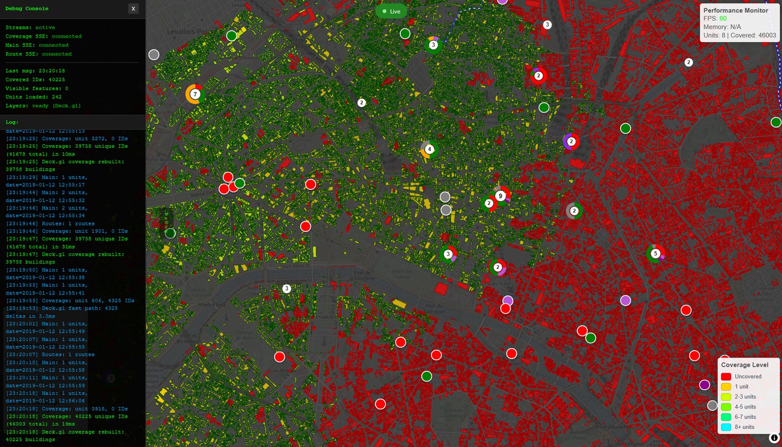
Emergency dispatchers in Paris worked from a map of 77 sectors. Seventy-seven polygons for a city of three and a half million buildings, drawn once and rarely revisited. Everything finer than that — which streets are covered right now, whether moving one station would help — lived in the experience of the person on the desk.
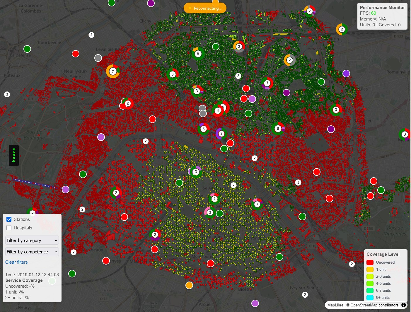
What replaced them. Every building coloured by how many units can actually reach it inside the response budget — red uncovered, cyan eight or more. Circles are stations, numbered by units available.
I first modelled that problem for my engineering thesis in 2017. I have kept coming back to it since, and it eventually became a working platform. This is what it takes to answer the question honestly.
Coverage is not a circle
The intuitive picture is a radius: draw 2 km around each station, colour it in, done. It is wrong in the way that matters. A unit 400 m away across a river is not 400 m away. A building behind a rail cutting can be six minutes from a station its neighbour reaches in ninety seconds.
Answering "is this building covered?" honestly means computing an actual road-network travel time from every candidate vehicle to that building — and computing it again every time a vehicle moves. For Île-de-France that is 3.3M buildings against 464k road segments, continuously.
Route queries also have to be fast in absolute terms, not just asymptotically. Contraction hierarchies solve that: the graph is preprocessed once, offline, into a contracted form where shortest-path queries collapse to a fraction of the work. Built once with RoutingKit, saved to disk, loaded at startup, then queried millions of times.
The part nobody warns you about
Even with sub-50 ms routing, the naive shape of the problem does not survive contact with reality. If every building is a routing target, each vehicle position update means 3.3M shortest-path queries. No amount of preprocessing saves that.
So you never route to a building. You route to the road graph — 464k segments instead of 3.3M targets, a reduction of roughly seven to one — and you attach the buildings to the roads offline, once, with a spatial join: each building centroid is matched to its nearest road segment through an R-tree index, producing a segment → [building ids] mapping. In the Île-de-France build, 2.5M buildings resolve onto 389k segments.
At runtime the engine computes reachable road nodes, thresholds them against the travel-time budget, marks the ways whose endpoints are covered, and then fans out through that precomputed mapping to say which buildings those ways carry. The expensive geometry happens once, offline. The online path is a shortest-path run, a threshold, and a lookup.
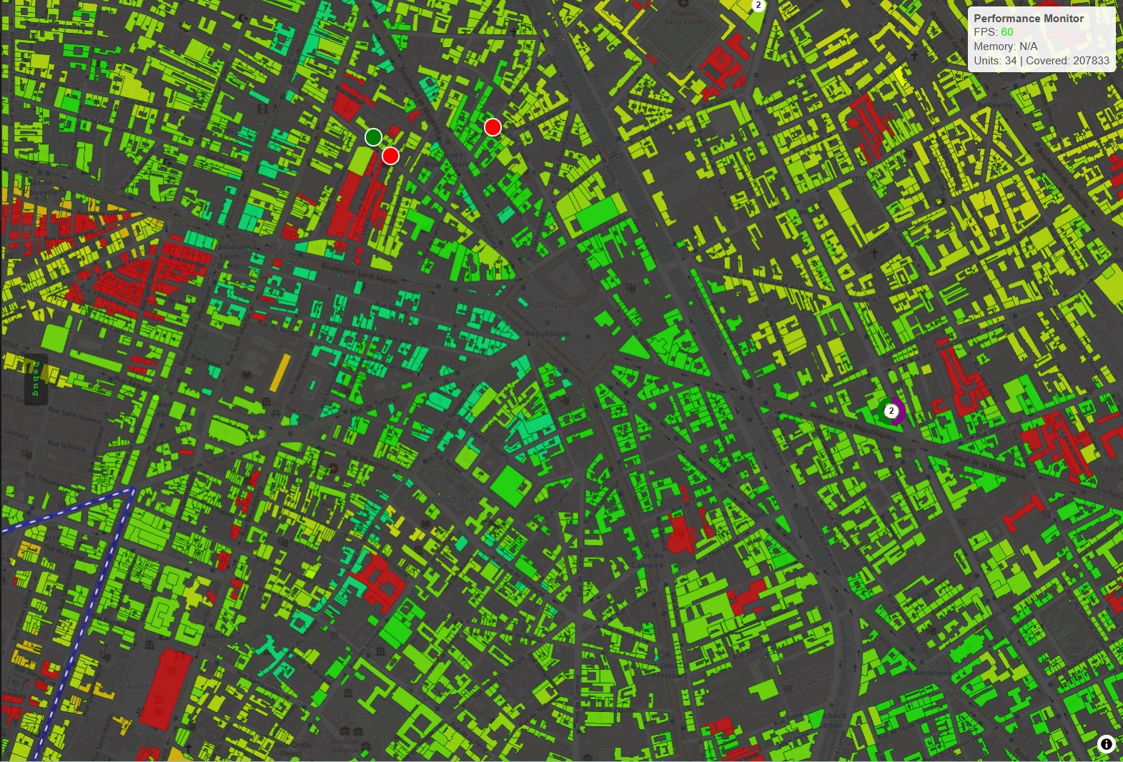
Zoomed in, the unit of analysis is a single building — not a sector, not a radius. Two neighbours can sit on different sides of the threshold because the roads that serve them differ.
flowchart TB
    subgraph offline [Offline, once per city]
        PBF[OpenStreetMap .osm.pbf] --> G[Road graph<br/>head · tail · travel_time]
        G --> CH[Contraction hierarchy<br/>built and saved]
        PBF --> B[Building footprints]
        B --> RT[R-tree spatial join]
        G --> RT
        RT --> MAP[(segment to building ids)]
    end
    subgraph online [Online, per position update]
        POS[Vehicle position<br/>via Kafka] --> Q[One-to-many query<br/>on pinned targets]
        CH --> Q
        Q --> GPU[CUDA: threshold nodes<br/>mark ways · count units]
        GPU --> FAN[Fan out through mapping]
        MAP --> FAN
        FAN --> R[(Redis)]
        R -- SSE --> UI[Map repaint]
    end
When the data structure stopped being enough
For a long time the answer to every performance question was the data structure, not the hardware. Contraction hierarchies made routing cheap; the offline join made the fan-out cheap.
Then the per-building work became the bottleneck. Thresholding nodes against a budget, marking ways, incrementing a per-way counter of how many units cover it — all of it embarrassingly parallel, all of it running in sequential CPU loops over millions of elements.
That is what CUDA kernels are for. Four of them: threshold the nodes, mark the ways, increment capacity, aggregate per way. With automatic CPU fallback, because a platform that only runs on a GPU machine is a demo, not a platform — without a CUDA device the backend logs the fallback and keeps working, just slower.
I resisted the GPU for a while, on the principle that reaching for hardware usually means you have not thought hard enough about the algorithm. That principle was right until it wasn't: once the routing was genuinely cheap, the remaining work really was a parallel scan, and the honest answer was the GPU rather than more CPU.
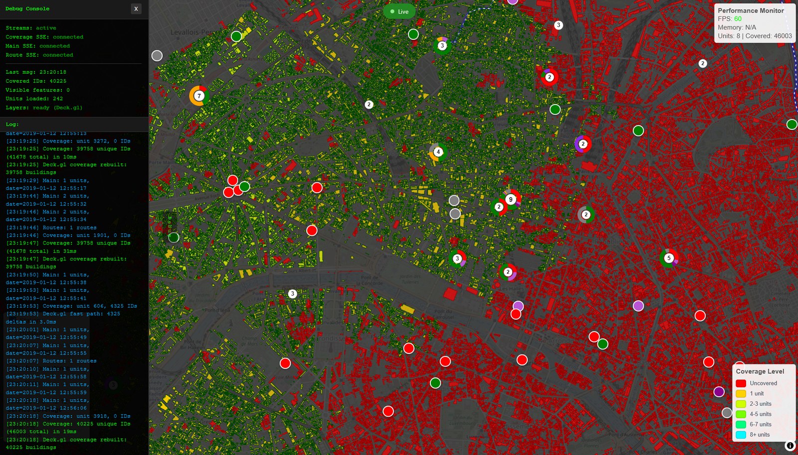
The claim, made checkable. Debug console open: three SSE streams connected, 242 units loaded, each position update rebuilding coverage — 40225 unique IDs (41678 total) in 10ms, then 46003 total in 19ms — with a delta fast path pushing 4325 deltas in 3.0ms, held at 60 FPS.
A ten-minute target is not the same area at 3 a.m.
Coverage thresholds are usually written as a constant: ten minutes, and that is the standard.
But the ten minutes include mobilisation — the delay between a crew being alerted and the vehicle actually moving — and mobilisation is not constant. It is materially longer at night, when crews are asleep, than mid-afternoon. Hold the total target fixed and the travel budget shrinks accordingly, which means the genuinely covered area shrinks with it.
So a gradient-boosted model produces an hourly mobilisation profile, and the travel-time budget is adjusted hour by hour. The map at 03:00 shows less coverage than the map at 14:00 for the same fleet in the same positions — which is not a bug, it is the point.
Honest status
This is an R&D prototype. It runs on five cities — Paris/Île-de-France, Annecy, Andorra, Vaduz, San Marino — the pipeline is city-agnostic, and a new city is a data run rather than a rewrite. It has never been deployed in live operations, and its full operational value belongs to large emergency services rather than to me.
It was built solo, unofficially, across nine intermittent years around day jobs. An earlier phase was presented at Mission Critical Technologies during London Tech Week 2019.
The source is public: github.com/Ben74Builds/coverage-management-system. No operational data ships with it — the road network comes from OpenStreetMap and all vehicle activity is produced by a simulator.
What I would defend in an interview
The offline/online split. Almost every hard number in this system — sub-second updates over millions of buildings — comes from deciding what can be precomputed and never touched again, rather than from making the runtime faster. The contracted graph and the segment-to-building mapping are both the same move: pay once, in a batch job nobody is waiting on, so the loop that runs while someone is watching does almost nothing.
The second thing I would defend is the dynamic threshold, because it is the one place where the model contradicts the official picture. A service that reports a fixed ten-minute coverage figure is reporting an average. The map that changes hour by hour is less flattering and more true, and I would rather ship the second one.
Stack: C++17 · RoutingKit · CUDA · Apache Kafka · Redis · PostgreSQL · Python · LightGBM · MapLibre GL JS · deck.gl · Docker · Server-Sent Events · OpenStreetMap